TIL: SORT, UNIQUE, VSTACK
How to use three formulas to combine and sort the unique values from two different lists (arrays)
Imagine two very long lists of unique codes (names, id numbers, any unique identifier). You need a single list of the unique codes. There are several approaches but I learned about VSTACK recently, have wanted to use it, and had to look it up again to apply it, so I am writing this as a TIL - today I learned.
Use the two lists to combine (VSTACK) them into a single list of unique values (UNIQUE) that is sorted (SORT).
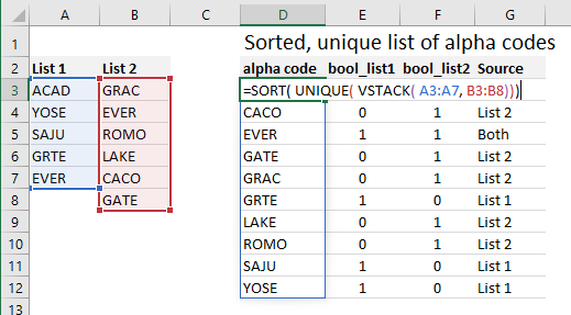
In the screen shot, the array formula in cell D3 combines these three Excel functions to produce the sorted list of unique alpha codes. Two adjacent Boolean columns give a 1 or a 0 depending on whether the alpha code is from list one or two. ISNUMBER and MATCH are used with double unary characters to return the 1’s and 0’s. A value of 1 indicates it was from that list; a value of 0 indicates it was not.

The final column, Source, uses an IF formula and the Boolean columns to indicate where the alpha code appeared–list 1, list 2, or both lists. Careful readers will note that EVER appears in both lists and the IF formula correctly identifies that in column G.
Formulas
D3: = SORT( UNIQUE( VSTACK(A3:A7, B3:B8)))
E3: = --ISNUMBER( MATCH( D3#, $A$3:$A$7, 0))
F3: = --ISNUMBER( MATCH( D3#, $B$3:$B$8, 0))
G3: =IF(AND(E3, F3), "Both", IF(E3, "List 1", "List 2"))
Functions
VSTACK - Appends arrays vertically and in sequence to return a larger array.
SORT - The SORT function sorts the contents of a range or array.
UNIQUE - The UNIQUE function returns a list of unique values in a list or range.
ISNUMBER - checks whether a specified value is a number (TRUE) or not (FALSE)
MATCH - The MATCH function searches for a specified item in a range of cells, and then returns the relative position of that item in the range.
IF - makes logical comparisons and can have two results, one if the comparison is TRUE and the other if the comparison is FALSE.