Persistent Default Values in An Excel Model
Hat tip to my colleague, Dan Schriever, for this post sparked by one of his posts on Yammer.
Via Dan:
Attached is an example of a method I use to provide persistent default values. That is to say, sometimes, I want to provide a default value for an input in case the User chooses not to provide one (or simply doesn’t have better information). An example might include a default inflation rate, unit cost, start year, discount rate, or scoring weight.
While I can always prepopulate a cell with a default value, if the User overwrites it, then deletes his/her value, the resulting blank cell may cause an error or misleading result in my output. Using this method, when the User deletes his/her entry from an input cell, the model will revert to the default value.
This same functionality can be acheived differently using VBA. However, this method helps to provide a finished look & feel in cases where VBA is not permitted.
I like this and the implementation. The Excel file explains things clearly. In order to pull this off there are several tricks employed in the set-up including:
- Use of the REPT(), TEXT(), ISBLANK(), and ISNUMBER() Functions
- Use of Custom Number Formatting
- Use of formulas that are somewhat hidden to the end user
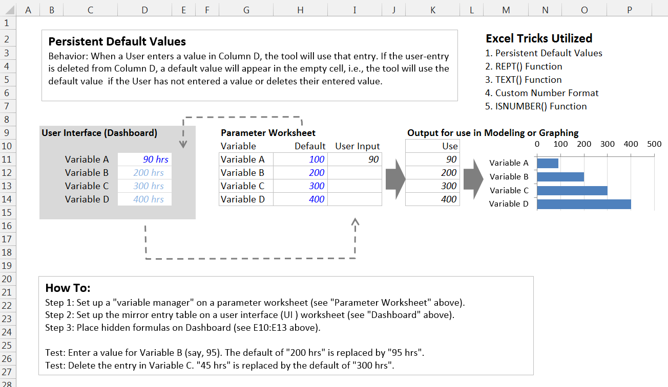
Download the file and investigate. I am not going to discuss everything here but the key piece of it all in my mind are the formulas in cells E10:E13 which are really responsible for the persistent default values being displayed to the user. Examining these formulas and understaning what is going on in addition to the other pieces described in the file are key to the whole trick.
The formula in cell E10 of this workbook reads:
= TEXT(H11,"#,##0") & " hrs" & REPT(" ",11)
To breakdown that equation and understand what is going on we first must understand that the ampersands (&) are being used to concatenate the results of the TEXT() and REPT() functions with a text string of “ hrs” in the middle. So in English, the result of the above equation could be stated as:
- The result of the TEXT function, “ hrs”, and the result of the REPT function combined into a text string
The TEXT Function
Now let’s review the TEXT() function and recall that it takes an input (cell H11 here) and formats that input according to the desired output format (Excel refers to this as the format_text). In this case the codes inside the quotation marks for the output format are telling Excel to display the value with standard number formatting with a comma. The TEXT function in this case is telling Excel to take the value in cell H11 and display it with number formatting. Appended to that nicely formatted number via the ampersand is the text string “ hrs” and appendend to that is the output of the REPT function.
The REPT Function
The REPT function in Excel is very straightforward. It takes an input and repeats it a specified number of times. In this example the input is a space designated in the formula as “ “ and the number of times to repeat that is 11. So the REPT function is simply adding 11 spaces on to the end of our resulting text string. The number of spaces needed varies everytime this trick is employed; as developers we need to play with the layout and setup to get things right and adjust the number of spaces so things look visually correct to the end user. This is essentially pushing the result of the formula over into the adjacent cell. The formula resides in column E but becuase of the use of the REPT function the result will appear to the user to be located in column D.
Custom Number Formatting
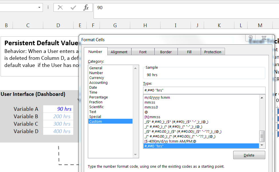
This is great; it is now readily apparent how the model is displaying the default values. What about when a user enters a value into one of the user entry cells (D11:D14)? We want to display their value with the appropriate unit of measure, the abbreviation for hours (hrs) in this case. If you place the cell selector in D11 and review the entry in the formula bar you will confirm that 90 has been entered but how then is Excel displaying 90 hrs? Custom number formatting is the second key to this process.
In the example here the custom number format has been applied as #,##0 “hrs” which tells Excel to display the number with a comma if necessary and the abbreviation ‘hrs’ at the end. See the picture below of the Format Cells dialog box.