Dynamic Data Validation in Excel
UPDATE: Preferred method described a week later in this post. It involves using the INDEX function on either side of the : range operator to define a named range that will be dynamic becuase it is based on the formula. I have left the following here for posterity.
The ability to have dynamic pick lists in an Excel model presents itself frequently enough that I am writing up two methods for achieving it. Specifically, I recently received a request to implement data validation with a dynamically changing pick list based on the data contained in each record. The client had a very large list that was to serve as the source for the pick lists but only a portion of the list was valid for a given record in the data table based on which field was tagged for that record. I realized pretty quickly that a named range defined with the OFFSET function might work even though the client approached us about developing a VBA macro based solution. Both were relatively straightforward but tricky enough that I thought it would be worthwhile documenting them and providing an example file.
In the example workbook, Dynamic Data Validation.xlsm, the data resides on a worksheet titled Data and is setup as a Structured Table with the name tbl_data. The required data validation is to occurr in colums J and K, SystemValue and Value respectively. The list used for data validation is stored on the worksheet titled PAR03-List (short for parameters) in a Structured Table with the name tbl_list.
For any building record in tbl_data that has the DomainID of BLDG we want the data validation in columns J and K of tbl_data to be just the 10 values for the BLDG DomainID from the tbl_list. If we are considering a trail record with a DomainID of TREADTYPE we want only the 8 tread type values from the tbl_list presented as data validation. Below are two methods for achieving this dynamic data validation.
Method 1: Named Range defined with OFFSET Function
The first method I used for column J relies on setting up Data Validation using the OFFSET, MATCH, and COUNTIF Functions and named ranges. The use of named ranges is important for making this dynamic in that if the user needs to add to or remove items from the pick list (tbl_list) having the named ranges setup this way will automatically capture the additions or subtractions with no other action.
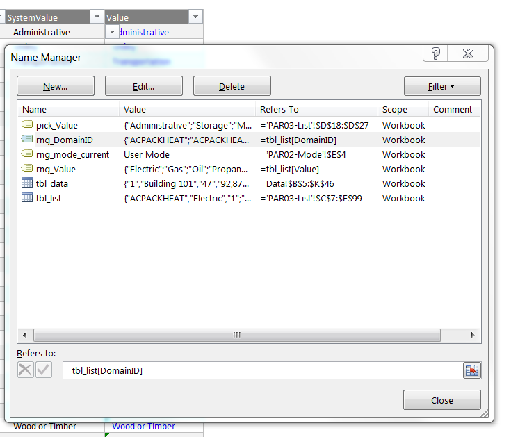
The two named ranges are for the DomainID and Value fields in tbl_list. I use the abbreviation ‘rng’ (short for range) at the start of the name with an underscore (_) and a description or value that is meaningful to finish the name. Reviewing the named ranges in the Name Manager shows
rng_DomainID = tbl_list[DomainID]
and
rng_Value = tbl_list[Value]
where I have defined both named ranges as pointing to the structured table references that are appropriate, DomainID and Value, in this case. There are a few other named ranges and the already discussed structured tables visible in the Name Manager as well but they can all be ignored for now.
Next it is important to understand the three functions being used to set-up the data validation - MATCH and COUNTIF are nested inside of OFFSET to produce the desired result. Let’s review OFFSET first. The OFFSET function returns a reference to a range that is a specified number of rows and columns from a starting cell or range of cells. Review the documentation for further information.
= OFFSET (reference, rows, cols, [height], [width])
The first three arguments - reference, rows, and cols, are all required. The final two are optional. For reference I have it set to the full list of Values in tbl_list as the starting range. Next determine how many rows down (or the offset) for the returned reference range to begin at and also the height of the returned reference range. MATCH and COUNTIF are used to dynamically determine these things.
So using the following for reference, rows, and height:
reference = rng_Value
rows = MATCH(I5, rng_DomainID, 0) - 1
height = COUNTIF(rng_DomainID, I5)
and substituting in the OFFSET function results in the final formula used for data validation (for cell J5):
= OFFSET ( rng_Value, MATCH(I5, rng_DomainID, 0) - 1, 0, COUNTIF(rng_DomainID,I5) )
A review of both the MATCH and COUNTIF functions may be helpful. The MATCH function searches for a specified item in a range of cells, and then returns the relative position of that item in the range. The COUNTIF function counts the number of cells in a range that meet a given criterion. As mentioned above MATCH is determing how many rows from the top of the reference range our new range should start and COUNTIF is determining the height of the new range.
In this workbook the MATCH function looks at the record’s DomainID field and goes to the list table (tbl_list) and finds which row that record’s DomainID appears and returns that row number as the result of the function. It is VERY IMPORTANT that the tbl_list be sorted alphabetically by DomainID in order for both methods described to work correctly. The COUNTIF function then determines how many times a record’s DomainID appears in the tbl_list so that the returned count acts as the height of the new range.
Put it all together with an example by considering what is happening for the record for Building 101. It has a DomainID of BLDG. Reviewing the tbl_list on the PAR03-List worksheet shows that BLDG appears in the 12th row below the header row but the OFFSET function is starting from cell D7 so subtract one to get that the BLDG section begins 11 rows below the reference. BLDG appears 10 times in the table so we need a range height of 10. Review columns M and N on the Data workhseet to see the calculations for each record for the MATCH (Rows from C7) and COUNTIF (Range Height) functions.
= OFFSET ( rng_Value, MATCH(I5, rng_DomainID, 0) - 1, 0, COUNTIF(rng_DomainID,I5) )

results in the following for Building 101:

= OFFSET ( rng_Value, 11, 10)
So the OFFSET functions in this example starts with the range (reference), rng_Value, and resizes it by going down 11 rows (rows) and making the range 10 rows high (height) - in this case the resulting range corresponds to cells D18:D27 on worksheet PAR03-List. Exactly what is needed for the data validation pick list.
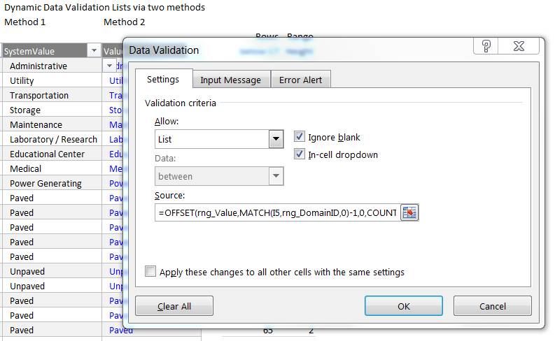
Reviewing the data validation for column J, SystemValue, of the Data worksheet shows it set to allowing values from a list with the source set as the OFFSET function and MATCH and COUNTIF for the arguments rows and height as described above. See screenshot above.
Method 2: VBA Macro dynamically changes named range based on user selection
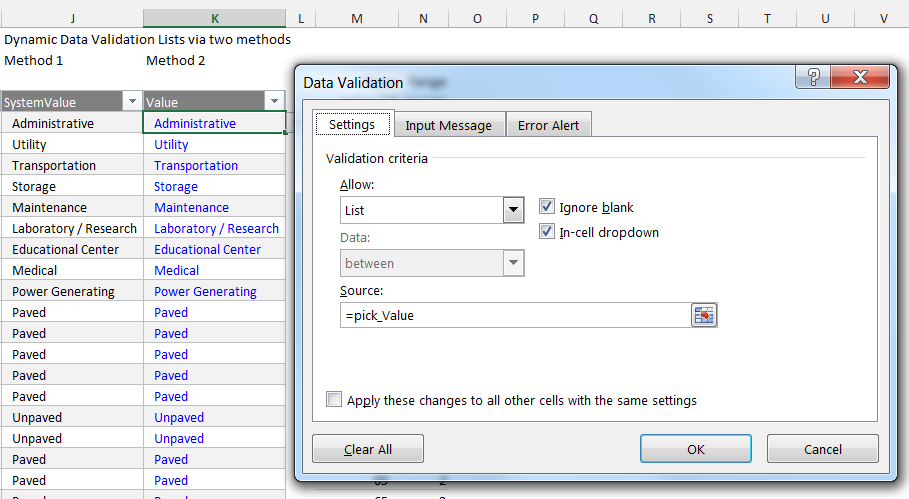
The second method used for the dynamic data validation and demonstrated in column K of the Data worksheet relies on VBA code which resides on the worksheet’s code module and watches for the user to select a cell in the target column which then triggers code to run that dynamically changes the definition of the named range pick_Value based on the DomainID for the selected record.
Review the screenshot below which shows how the data validation for this column is applied. It is set to allow values from a list with the source set as the named range pick_Value. The trick is that every time the cell selector is placed in column K of the Data worksheet and within the defined tbl_data range the VBA macro dynamically changes the definition of the named range. The OFFSET, MATCH, and COUNTIF functions are all being handled by VBA code. See the code black at the end of this post for the entire VBA code used to achieve this. I am not going to cover the code here.
Of course there are positives and negatives to each of these method. Some are explored below.
Pros
-
Method 1 is more straightforward to set-up for an average user. It only requires named ranges and a specific formula that is easily edited.
-
Method 1 has consistently applied data validation across the full data set at all time. Method 2 will not because at any given time the data validation is only appropriate for a subset of the data because the macro changes the range that the named range points to every time a user selects a different cell.
-
Method 2 is generally faster and will result in a lighter (file size and calculation speed) workbook than Method 1 (see con about volatile functions).
-
Method 2 may seem more straightforward to advanced users.
-
Because both methods are using a structured table reference for tbl_data it is very easy for the end user (or anyone) to add to the default list of approved values. The table will expand and contract accordingly and the named ranges will adjust as well.
Cons
-
Method 1 relies on
OFFSETwhich is a volatile function. Volatile functions are those whose results cannot be assumed to be the same from one moment to the next even if none of the arguments has changed. Excel reevaluates cells that contain volatile functions, along with all dependents, every time that it recalculates. In a large data set this method would significantly slow down the model because of this calculation overhead. -
Method 2 relies on VBA code which means the workbook must be macro enabled and the user sophisticated enough to figure out what is wrong and why things are not working as expected if macros happen to be or become disabled.
-
The table that acts as the source list (tbl_list) needs to be sorted alphabetically for either method to work. This could easily be addressed with additional VBA code to always sort the list immediately following user selection in the target column and then running the remainder of the existing code.
-
Users must be comfortable with intermediate to advanced topics in general to use either method:
COUNTIF,MATCH,OFFSET, VBA, macro-enabled workbooks, structured table references, and named ranges defined with structured table references are all more advanced than entry level Excel.
VBA Code for Method 2
Note that this code needs to reside on the Data worksheet’s code module and not in a standalone code module.
Private Sub Worksheet_SelectionChange(ByVal Target As Range)

    Dim rng_click As Range
    Dim rng_DOMAINID As Range
    Dim rng_VALUE As Range
    Dim int_row_offset As Integer
    Dim int_rows_count As Integer

    Set rng_click = Target.Cells(1)
    Set rng_click = Intersect(rng_click, Range("tbl_data[Value]"))

    If Not rng_click Is Nothing Then
        'Read DOMAINID and VALUE into VBA memory

        Set rng_DOMAINID = Worksheets("PAR03-List").Range("rng_DomainID")
        Set rng_VALUE = Worksheets("PAR03-List").Range("rng_Value")

        'If two cells to the LEFT of Target <> "" Then set pick list ELSE pick list is blank

        If rng_click.Offset(0, -2).Value <> "" Then
            'Find first row or offset and height of the range for the pick list

            int_row_offset = WorksheetFunction.Match(rng_click.Offset(0, -2).Value, rng_DOMAINID, 0) - 1
            int_rows_count = WorksheetFunction.CountIf(rng_DOMAINID, rng_click.Offset(0, -2).Value)

            'Set pick list range

            Set rng_VALUE = rng_VALUE.Offset(int_row_offset).Resize(int_rows_count)
            ActiveWorkbook.Names.Add Name:="pick_Value", RefersTo:="='PAR03-List'!" & rng_VALUE.Address

            Else

            'Set pick list so it is blank, NOTE: Domain Checker:D1 must be BLANK (empty)

            Set rng_VALUE = Nothing
            ActiveWorkbook.Names.Add Name:="pick_VALUE", RefersTo:="='PAR03-List'!A6"
        End If
    Set rng_click = Nothing
    End If
End Sub