Preferred Method - Dynamic Data Validation in Excel
There is almost always more than one way to do something in Excel and sometimes an even better way. Last week after writing up two methods for dynamic data validation in Excel a colleague pointed out that a non-volatile solution could use the INDEX function and the range operator to define a named range that would be dynamic because of the formula used to define it. Another colleague pointed out that a simpler example was in order. The file, Dynamic Picklists.xlsx, is that example.
The tip to use INDEX on either side of the range operator (:) is brilliant. When I tested it and showed it to another colleague he remarked “this is evil black magic” and I countered that I thought it was more of a Jedi mind trick (‘these are not the droids you are looking for’). Bad references to movie quotes aside, in order to even use the range operator we need something on either side of it to tell Excel where to begin and end the range - and this is where the power of INDEX shines and indeed edges toward evil black magic.
A web search and review of material on the INDEX function shows that many others recognize it’s powers. Daniel Ferry over at the excellent Excel Hero Blog sings the praises of the INDEX function in his post titled ‘The Imposing Index’ (emphasis following mine):
Now that might be surprising considering the function’s humdrum name, but please pay close attention, because INDEX is one of the magical secrets of how to use Excel! So what’s so great about the INDEX function? It’s nonvolatile, sprightly, agile, and versatile. Excel INDEX can return one value or an array of values; it can return a reference to one cell or to a range of cells. INDEX works well on either side of the three Reference Operators – the colon, the space, and the comma.
INDEX can be used to create a dynamic range, and not only is it nonvolatile, it is way faster than either OFFSET or INDIRECT. In fact, the improvement in performance is so great that INDEX should be the foundation of all dynamic ranges in professional models.
Ferry’s post provides confirmation that the tip from my colleague was the way to go and it strongly recommends this approach as the foundation for dynamic ranges in professional models. To set up dynamic data validation with this method requires a named range that is defined using INDEX on each side of the range operator. The first INDEX function dynamically determines the beginning of the desired range and the second INDEX function determines the end of the desired range. Recall that the range operator (: colon) is one of three reference operators and that it is defined as:
Range operator, which produces one reference to all the cells between two references, including the two references
Range operator is exactly what is needed in this method. Placing the two described INDEX functions on either side of the range operator will return the desired range.
In the following screen shot from the example file we see the data table has columns for ID, Class, and Species and the end user should be able to select the desired Class and then get the related Species pick list in the adjacent cell. Both static pick lists are contained on the TBL02-Species worksheet and all tables in the model are structured tables.
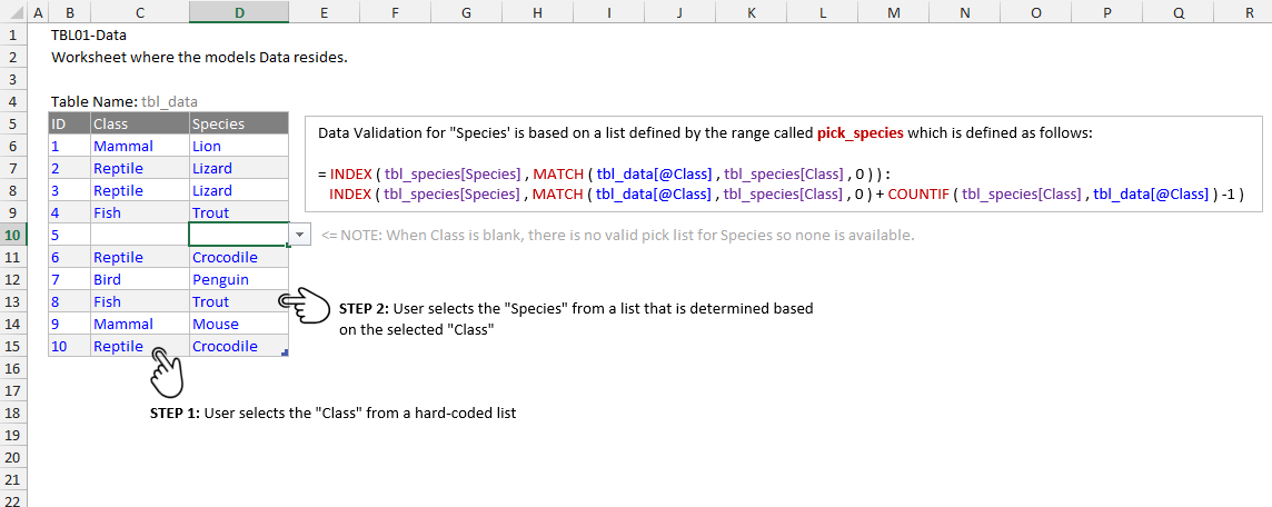
Reviewing the INDEX functions on each side of the range operator will illustrate how the final range is being determined. Note that in the screenshot above and the example file the left side of the equation is listed first then the colon and the right side of the colon is listed next on its own line. The INDEX function on the left side of the colon (range operator) is:
= INDEX (tbl_species[Species], MATCH(tbl_data[@Class], tbl_species[Class],0) )
Recall that INDEX returns a reference of the cell at the intersection of a particular row and column in a given range. By using MATCH to define the row and using the species list, tbl_species[Species], as the reference range for INDEX we get the reference to the start of the range we ultimately want. MATCH is simply looking at a particular record’s selected Class and then returning the row number of that class from the Class list, tbl_species[Class].
The INDEX function on the right side of the colon is slightly more complex because it also uses COUNTIF. We already know the starting row of the desired range (from the INDEX function on the left side of the colon) but we need to determine the final row. By adding the COUNTIF portion to the end of the equation we arrive at the final row. The COUNTIF is determining how many times a record’s Class appears in the Class list, tbl_species[Class].
The final formula used to define the named range pick_species:
= INDEX(tbl_species[Species],MATCH(tbl_data[@Class],tbl_species[Class],0)) : INDEX(tbl_species[Species],MATCH(tbl_data[@Class],tbl_species[Class],0) + COUNTIF(tbl_species[Class],tbl_data[@Class]) - 1)
Considering a specific example will further illustrate how the formula for the named range is working. For record ID 1, the selected Class in the example workbook is Mammal. The first Species in the list for Mammal is Lion and Mammal appears 5 times in the Class list but since we are already starting on the Lion row of the Species list the formula only needs to go down 4 additional rows to arrive at the bottom (Mouse) so that is why there is a minus one after the COUNTIF on the right side of the range operator. Substituting all of this into the formula for the pick_species named range:
= INDEX(tbl_species[Species], MATCH (Mammal, tbl_species[Class],0)) : \n
INDEX(tbl_species[Species], MATCH (Mammal, tbl_species[Class],0) + COUNTIF(tbl_species[Class], Mammal) - 1)

evaluates to

= INDEX(tbl_species[Species], 1 ) : INDEX(tbl_species[Species], 1 + 5 - 1)

evaluates to

= Lion : Mouse
The formula returns a list starting with Lion and ending with Mouse. Exactly what is needed.